GrAPPA:Graph Algorithms Pipeline for Pathway Analysis

What you will learn from this tutorial.

This tutorial covers typical usage of the different tools available under GrAPPA. By the end of this tutorial, you should be familiar with how to upload .CEL data to GrAPPA, normalize the .CEL data and place the results in a tabular format, extract correlations from the data, and use the resulting correlated data on one of GrAPPA's graph decomposition algorithms.

Uploading Data

Although GrAPPA can be used to handle any data that can be placed in a tabular format, one of the most common uses for GrAPPA has been the analysis of biodata. The Gene Expression Omnibus (GEO) is a database which maintains a wealth of biodata that can be used on GrAPPA. For this tutorial, we shall analyze .CEL data obtained via GEO from a study on human patients with cerebral palsy. These files can be found here.

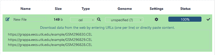
Once you have downloaded the .CEL files, you will need to upload them for use on GrAPPA. To upload the files, Click on Upload File under the Get Data tab on the left-hand side Tools panel. This will display the upload file screen in the center panel. Under File Format, be sure to set the format of the file to .CEL. Then, click on the Choose local file button to search for the files on your computer or upload from url. Once a .CEL file has been specified, click on the Start button at the bottom. Repeat until all the .CEL files needed are uploaded. For this tutorial, I simply uploaded the first five .CEL files from the study.

GrAPPA supports many different filetypes, not just .CEL files. Here is a list of supported types:

bcl - A list of bicliques. Output by biclique.

bel - A bipartite edgelist. Compare el and kel. Used by biclique.

bmat - A binary matrix. Used by biclique.

cel - A CEL format produced by microarray software.

cl - A list of cliques produced by paraclique, maximum clique, or maximal clique.

el - A graph edgelist format. All lines are 2 columns separated by a tab character. The first line consists of the number of vertices and the number of edges. All following lines contain two vertex labels denoting an undirected edge between them.

gv - GraphViz format used as input to the graphviz tools.

kcl - A list of k-partite cliques. Outputted by k-partite clique enumeration.

kel - A k-partite edgelist. The only differences between a normal edgelist is that each group has its own size and the vertices must use contiguous integer labels.

kmat - A k-partite matrix. See the documentation for k-partite clique enumeration for more information. Allows the use of arbitrary string labels.

mat - A tab-delimited matrix file, with a header for the first row and first column.

tab - A tab-delimited table format. Short for "tabular".

txt - A plain ASCII text file

wel - A weighted edgelist. Similar to el, except that each edge ends with a tab and a weight. Most of the tools available here expect floating point values between 0.0 and 1.0 as weights.

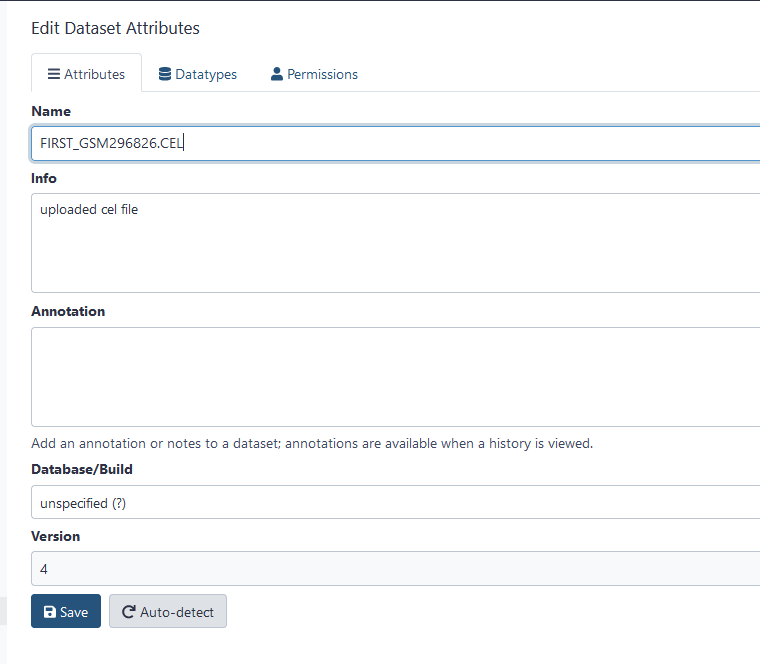
Notice that GrAPPA assigns a default name. Perhaps you wish to rename the file so it would have a more descriptive name. To do this, click on the pencil icon (next to the eyeball icon) of the file you wish to edit. A screen will appear in the middle panel labelled Edit Attributes. The name field appears at the top. Be sure to Save your changes once you are done editing.

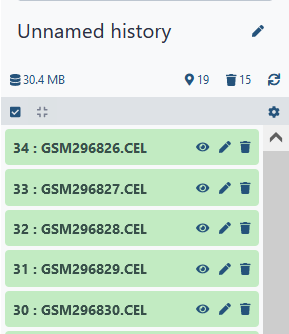
Tip: Some processes, including uploading files, may take a bit of time. If a process doesn't complete immediately, periodically click on the Refresh button to update the status of each process. This is especially useful for some time consuming tasks, such as correlation and graph decomposition.

Normalization

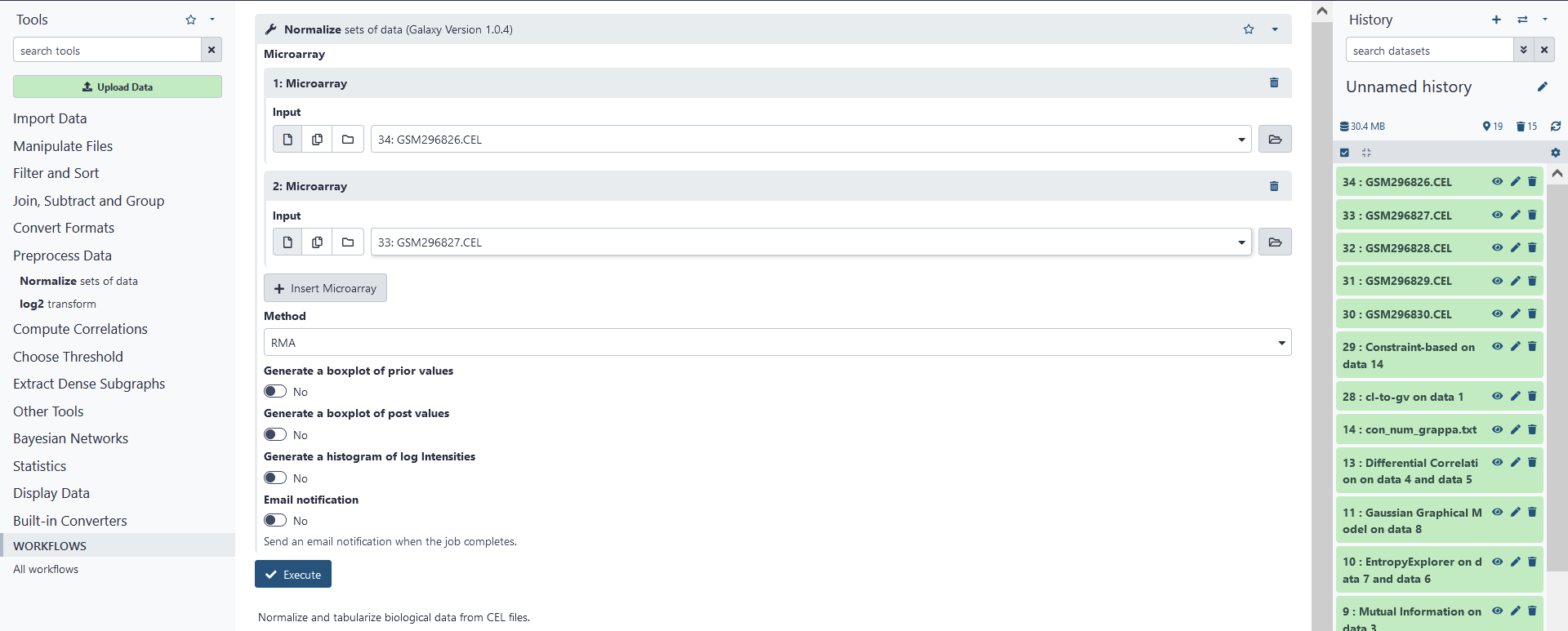
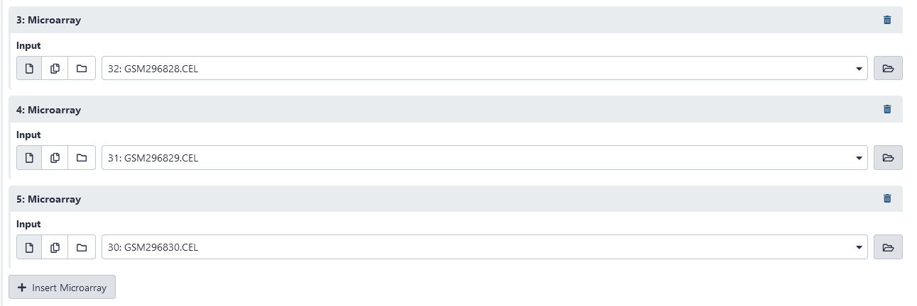
Now that we have uploaded our .CEL data, we need to compile the data into a single tabular file and normalize the values for further analysis. First, we must specify the microarrays (.CEL files) that we wish to compile into a single .TAB file. We will go ahead and compile all of the .CEL files we have uploaded. First, click on Insert Microarray. This should add a new microarray with the options to select the input (.CEL) file used or to delete the microarray. Select the first .CEL file uploaded. Add new microarrays for the remaining .CEL files.

After the microarrays have been added, we must specify the normalization method we wish to use. We may do this under the Methods box. The methods available are either Robust Multiarray Analysis (RMA), or MAS5. A precise definition of these normalization algorithms is beyond the scope of this tutorial. So, for our purposes, we will simply stick with RMA.

Once you have compiled the microarrays and selected a normalization method to use, click on the Execute button.

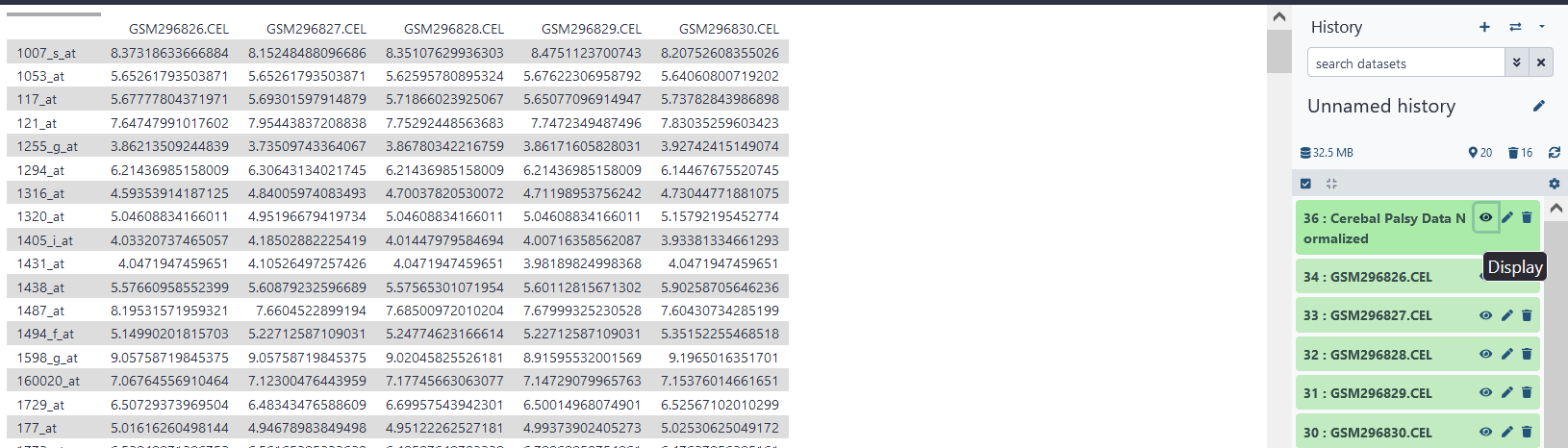
After normalization has completed and the .TAB file has been created, you may view the contents of the file. To view the contents of a newly created file, click on the eyeball icon directly to the right of the name of the file.

Correlation

Now that we have compiled and normalized our data, we will need to find correlations within our data in order to construct a graph. To do this, click on Pearson Correlation under the Correlation Matrices tab. As our input, we will use the normalized .TAB file we created previously. However, since there are a lot of row variables included in the .TAB file, and many of these variables appear to be highly correlated, for the purposes of this tutorial, I have truncated the .TAB file to only include the first 1000 normalized variables. Running correlation analysis on the original file would take a relatively large amount of time and possibly create a huge file. Be careful when running correlation analysis!

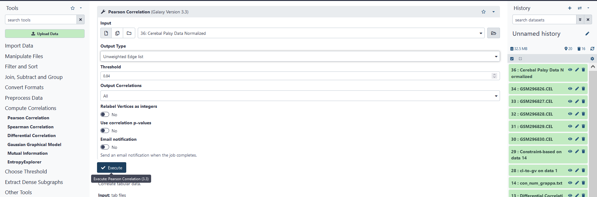
Under output, we have three choices, either a frequency histogram, a weighted edgelist (.WEL file), or an un-weighted edgelist (.EL file). The frequency histogram is simply a text file including the number of variables that fall within a correlation interval (these intervals range from -1.0 to 1.0 in increments of 0.01). The weighted edgelist is a DIMACS representation of a graph with undirected, weighted edges. The un-weighted edgelist is the same, except the edges have no weights. Since we are interested in constructing a graph, but we do not need the weights of the correlations, we shall choose an un-weighted edgelist as our output.

For weighted and un-weighted edgelists we have a few additional options. We can change the threshold, choose which types of correlations we consider (only positive, only negative, or all), relabel the vertices of the graph (the row variables of our .TAB file) as integers, and choose to use correlation p-values instead of correlation values to construct edges. For our purposes, we shall simply use the default values of these options. Click on Execute to run correlation analysis on the .TAB file, which will create a .EL file.

If you are not sure which threshold to use, you can use spectral threshold under the Data Preparation tab. For those interested, the correlation techniqued used for our analysis is Pearson correlation.

Graph Decomposition

There are many different graph decomposition tools available under GrAPPA. Note that all of these tools are used to solve NP-hard problems, which means that the computation time needed grows exponentially with the size of the input. Take this in to account when you use GrAPPA!

For this tutorial, we shall try to find all paracliques included in the graph we had constructed earlier. A paraclique is a densely-connected subgraph that is almost a clique, but is missing a few edges. Paraclique analysis is especially useful when dealing with noisy data.

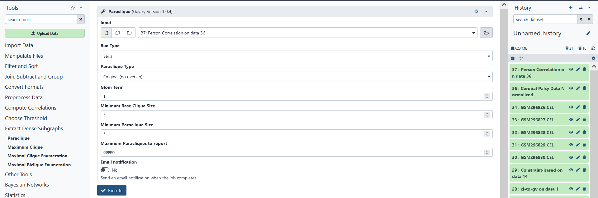
First, click Paraclique under the Clique Computation tab. Then, for Input choose the un-weighted edgelist file created during correlation analysis. The other options for paraclique include the Run Type, Paraclique Type, Glom Term, Minimum Base Clique Size, Minimum Paraclique Size, and Maximum Paracliques to Report. For our purposes, we shall keep these options as they are. Click on Execute to create a file containing a list of paracliques according to the options specified.

Summary of paraclique options:

Run Type: Parallel runs are sent to Newton to be processed while serial runs are handled locally. The process of sending jobs to Teragrid introduces delays that will not be experienced by serial jobs. As such it is recommended that you run small/fast jobs as serial and large/long jobs as parallel.

Original vs Accelerated Paraclique: For original paraclique, the glom term is fixed to the value specified, and growth stops when no more vertices can be added. For accelerated paraclique, the glom term grows by one for each pass through the graph, and growth stops when the paraclique meets the aggressiveness ratio (defined below).

Glom Term: If a potential vertex is disconnected from less than or equal to <glom term> vertices in the existing paraclique, it will be added to the paraclique.

Aggressiveness Ratio: Controls the growth of accelerated paracliques. When the current glom term is <agg ratio> percent or more of the paraclique size, growth is halted.

Overlap: With overlap set, paracliques are grown as with the non-overlapping algorithm, but then a second pass is done to add in previously removed vertices (ie vertices used in other paracliques).

Maximum Paracliques to report: The maximum number of paracliques to report. This is useful for restricting the output size and runtime. Use 0 to report unlimited paracliques.

Note that the graph created during correlation analysis can also use the Maximum Clique, Maximal Clique, and Dominating Set tools, since these all take .EL files as input.

Visualization

GrAPPA contains tools that can convert files to the GraphViz .GV format as well as display these graphs using a preferred layout (e.g. dot, neato, fdp, circo and twopi). However, care must be given when dealing with graph visualization, as very large graphs can take a very long time to generate formatted pictures. If you know that the results of graph decomposition yield a very large graph (or series of graphs), it may be wise to download the graph and use more sophisticated tools to generate very large visualizations.

Contact us

Many tools are not covered in this tutorial. If you have any questions, feel free to contact us. Email us: grappa@utk.edu